Introduction
Phrase mining is the process of utilizing automated programs for extracting important and high-quality phrases from bodies of text. These phrases can be used in a variety of ways, from extracting major ideas from customer reviews or key points from a scientific paper. However, phrase mining has historically been done with complicated linguistic analyzers trained on specific data, meaning that it is difficult to expand to a larger scope without significant additional human effort. As a way to mine phrases in an expandable way, in any language or domain, AutoPhrase was created. With AutoPhrase, it is possible to input any text corpora without the need for human labels, allowing for much faster extraction of phrases in a variety of documents.
With that in mind, we utilized AutoPhrase to extract the phrases from a database of 3,079,007 computer science research papers aggregated from 1950 to 2017. With this, we can trace the evolution of key ideas through the history of computer science, as well as find which ideas were most common in what years. Additionally, we used the extracted phrases as data to construct a classification model for finding what year a paper belongs to based on its key phrases as a way of showing how strong the connections are between ideas and time.
Data
- DBLP Citation Network Dataset v10 (4.08 GB)
- Four .json files containing information on 3,097,007 papers
Exploring the data
The original DBLP V10 data set we utilized for our project contains 3,097,007 total papers. However, during data processing, 530,394 were filtered out due to empty abstracts, as well as 82 others due to invalid year values. That leave us with 2,548,531 papers ranging from 1968 to 2017.
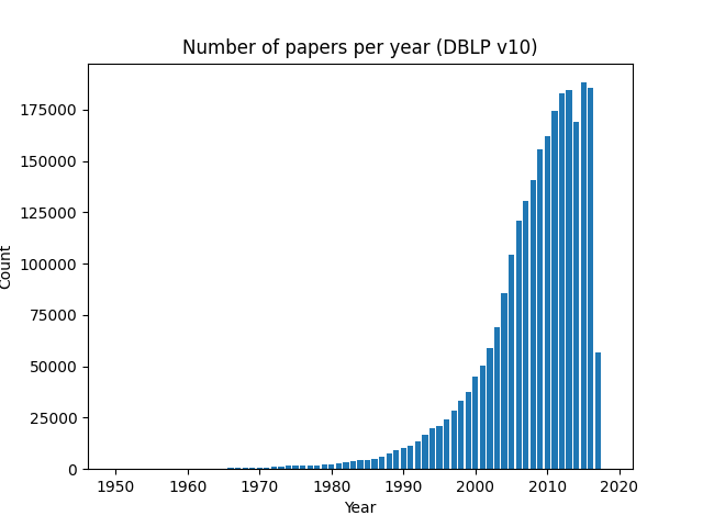
The number of papers has increased exponentially in recent years as the Computer Science field has grown in popularity and complexity. The last year in the graph (2017) is lower than the previous due to the dataset being published before the year was over. Overall, we can see that the number of papers per year strictly increases, with an exception in 2014 and 2017.
Data preparation
AutoPhrase has two functions that can be run. Phrase mining and phrasal segmentation. In order to perform the phrase mining step, a single .txt file is required. Once phrase mining is complete, a segmentation model file is generated that can be used to segment any .txt file, including the same input .txt file.
As a result, we processed the DBLP dataset from it’s original .json format into a .txt format. Since we want to analyze how phrases change over time, the information for each paper (title + abstract) is grouped based on their year range. We decided to group years together in intervals of 5, as a single year may not be a significant marker of change in the field overall. By looking at the years in groups of 5, we can obtain a clearer picture on the general trend of phrases and the change over a longer period of time.
All years are grouped in intervals of 5 years, except for the last years in the dataset (2015-2017) and the beginning years of the dataset (1950-1959). We decided to group the earlier years together as there are not many papers in the earlier years, as shown in the graph above.
Results
Phrase mining results
AutoPhrase’s phrase mining step was ran on each year range’s .txt file, containing all of the paper’s titles and abstracts. Separating out the dataset into year ranges is necessary, as phrase mining on the entire dataset will prevent us from associated a phrase with a specific year or year range. By having separate files for each year range, we know what phrases and phrase qualities are associated with a specific year range.
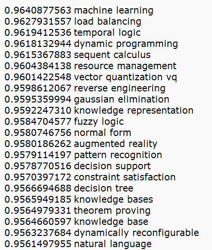
Phrase mining returns a .txt file containing a list of extracted phrases, along with their associated phrase qualities. Phrase quality ranges from 0.0 to 1.0, with 1.0 being the highest quality. Phrase mining can identify both single-word and multi-word phrases in the input text data. We found that the most common phrase length was two words long.
For further processing, we consolidated the phrase mining results for each year range into a single .csv file containing information on each phrase, its associated phrase quality, and the year range it was found in.
Phrasal segmentation results
The phrase mining step also outputs a segmentation model file, which can be used to segment any .txt file. By using the segmentation model to segment the original input text, AutoPhrase will mark any identified phrases with phrase markers.
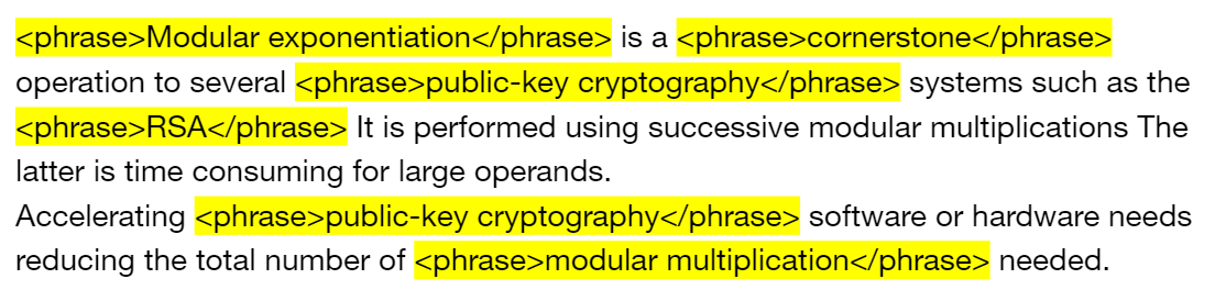
The figure above shows an example of what phrasal segmentation does to text data. Any mined phrases with be marked with phrase markers. The phrase markers and phrases are highlighted in this screenshot for clarity. By processing the phrasal segmentation results, we can extract the marked phrases and group them together. This allows us to see the phrases mined by AutoPhrase on a per-paper level. For instance, with the example, if we consider it the text for a single paper, we can see that it contains the phrases: modular exponentiation, cornerstone, public-key cryptography, and RSA.
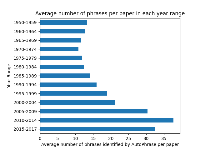
This chart visualizes the average number of phrases identified by AutoPhrase for each year range. From the phrasal segmentation results, we are able to identify the phrases contained in each paper in the dataset. We can then take the average number of phrases identified per paper, and graph that information.
Here, we can see that the number of phrases per paper changes drastically depending on the year range. This can be due to factors like average length of input papers for that year range, but could also be dependent upon the range of phrases displayed within that range. A year range with more phrase variety could have less phrases show up per paper due to the lower average scores of the phrases causing them to be excluded from our high-quality phrase list.
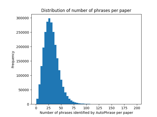
This histogram shows the distribution of the number of phrases identified across the entire DBLP dataset. Overall, the number of phrases in a paper can vary widely, but the vast majority lie between 15 and 50 phrases.
Most popular multi-word phrases over time
| 1950-1959 | 1960-1964 | 1965-1969 | 1970-1974 | 1975-1979 | 1980-1984 | 1985-1989 | 1990-1994 | 1995-1999 | 2000-2004 | 2005-2009 | 2010-2014 | 2015-2017 |
|---|---|---|---|---|---|---|---|---|---|---|---|---|
| operations research (82) | pattern recognition (27) | sequential machines (85) | pattern recognition (165) | natural language (253) | natural language (494) | expert systems (782) | neural network (2504) | neural network (4977) | neural network (6001) | web services (12672) | cloud computing (16170) | machine learning (11254) |
| gaussian noise (16) | regular expressions (22) | pattern recognition (75) | linear programming (122) | pattern recognition (132) | signal processing (268) | natural language (770) | natural language (1089) | genetic algorithm (1700) | data mining (4901) | neural network (12314) | machine learning (14046) | big data (10885) |
| differential equation (12) | differential equations (21) | linear programming (71) | sequential machines (82) | computer graphics (128) | dynamic programming (204) | programming language (509) | expert systems (832) | image processing (1663) | web services (3543) | data mining (9980) | wireless sensor networks (12345) | social media (9504) |
| dynamic programming (8) | linear programming (19) | analog computer (58) | computer graphics (72) | linear programming (106) | pattern recognition (192) | user interface (495) | image processing (827) | software engineering (1430) | software engineering (3188) | wireless sensor networks (9382) | neural network (11381) | cloud computing (8373) |
| standard model (8) | sequential circuits (15) | sequential machine (54) | dynamic programming (69) | problem solving (104) | linear programming (174) | artificial intelligence (398) | distributed systems (799) | distributed systems (1414) | genetic algorithm (3115) | genetic algorithm (8088) | data mining (11235) | power consumption (6124) |
By processing the phrasal segmentation results, we can obtain the frequency of each phrase in each year range’s text. We specifically focused on the most frequent multi-word phrases across each year range in order to identify the most popular Computer Science topics in each period. We can see how the frequency of the top 5 phrases increases greatly over time, as more papers are published and topics of papers overlap. In the early years, there is a large focus on ’pattern recognition,’ as it is in the top 5 in all of the year ranges from 1960-1984. Over time, this changes, with topics such as ’neural networks’ and ’machine learning’ becoming more prominent. Ultimately, this table provides insight into the most frequent phrases across each year range, and it does reflect the changes in the field as it has matured.
Phrase network
Link to high-resolution, zoomable image
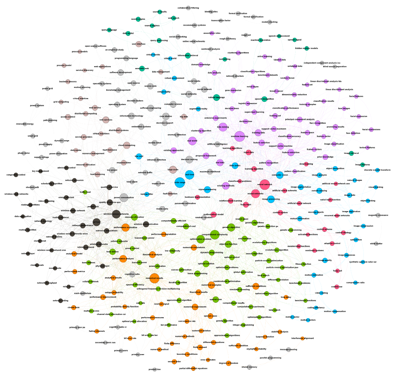
This network visualizes the relationship between phrases for all papers in the DBLP v10 dataset (across all years). Phrases with more more occurrences in the dataset are represented by larger nodes in the network. Nodes are connected based on their connections in the paper. The phrasal segmentation results allowed us to extract the phrases identified for each individual paper in the dataset. With this, we could calculate the number of connections each phrase had with each other. For example, if ’neural network’ and ’machine learning’ are in the same paper, we would count that as 1 connection. With more connections across papers, edges between nodes have a larger weight.
Node colors are determined by modularity, so nodes with stronger edges to each other will be grouped together. For instance, with the purple nodes, ’machine learning’ is the largest node, and we see other related nodes to that topic, such as ’decision trees’, ’support vector machines’, etc.
Phrase network by Year Range
Link to high-resolution, zoomable image
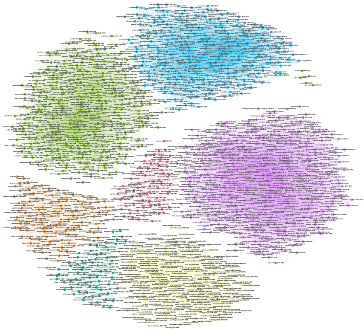
This network visualization takes the year range of each phrase into account. Rather than the node color being based on modularity, instead it is based on the year range the phrase belongs to. Although this network is more messy than the previous, it provides insight into the various phrases identified in each year range and their various connections. One fact to take into account is that the number of papers is much higher is recent years, so the frequency of phrases and their connections is much higher compared to earlier years. Steps were taken to normalize this difference across each year range and to only display the strongest and most meaningful relationships, but the number of nodes for each year range is not exactly equal.
Model
Model generation
One of our initial goals for this project was to create a classifier to predict the year of a random Computer Science paper in order to demonstrate how distinct phrases contained within certain years have the capability to identify what year of the input paper. For this, we attempted multiple types of models including a Jaccard-based predictor, a predictor using phrase overlap between years, as well as trained models using one-hot encoding. We were able to successfully create a model using a combination of the TF-IDF (Term Frequency-Inverse Document Frequency) text-vectorization and grouping of multiple years. Training on these features, we tested a variety of classifiers and settled on a Linear support vector classifier. We also used grid search to tune our hyperparameters.
Model results and output
From creating a train-test split on the phrase mining results and training the model, we were able to achieve a 79% f1 score on the test set. This is a small increase from an f1 score of 77% when taking the baseline tfidf model conducted with Linear Regression. While our model performs better than the baseline and much better than other models that we have tested, the performance isn’t could still use improvements. Ultimately, we realized that using phrases alone to predict what year range a paper belongs has limitations.
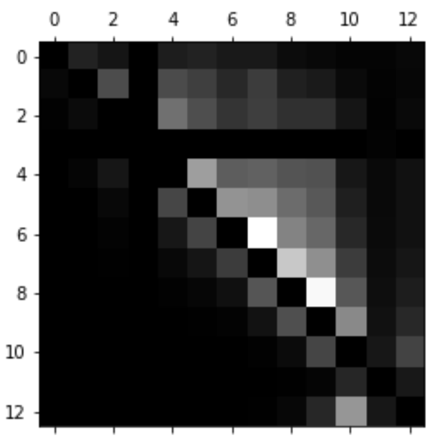
We performed additional analysis on our predicted results in the form of a normalized confusion matrix. This shows a visual representation of the prediction performance of each label compared to other labels. We have 13 categories of years with the oldest years starting at 0. The x-axis represents the true labels while the y-axis represents the predicted labels. Darker squares represent that there were a larger percent of true and predicted label pairs. This visualization shows that while we do have a good diagonal line representing correct predictions, the output of our model tends to predict much more recent year groups compared to the true label. This is likely due to our database’s paper count being imbalanced towards recent years.
Conclusion
After processing and exploring the DBLP v10 dataset, we were able to utilize both functions of AutoPhrase (phrase mining and phrasal segmentation) to extract meaningful data and explore the relationships between phrases further. We identified the change in phrases over time by looking at the most popular phrases for each year range. We analyzed the relationship between phrases on a per-paper level, utilizing the segmentation results, in order to create a network visualization. We analyzed this relationship in respect to time, visualizing the network of phrases for each year range. We created a classification model in order to predict the year range of a paper based on its phrases.